How to Use mpiv

The mpiv toolbox does not include image-reading and signal preprocessing in the program so the two sequential images (called image pair) have to be read in and background noise have to be subtracted from manually. The reason that an image-reading routine was not included and the PIV and post-processing programs are separated is for easy access and modification for pre-processing and post-processing. It is recommended that users write a simple program to read in a series of images if one needs to process more than a few images.

The first step is to read in an image pair(s). Perhaps the easiest way to read in images is using the imread command (see example below). After that, compute velocity vectors using mpiv.m. Finally, mpiv_filter.m is called to get rid of the stray vectors (replaced with NaN) and to fill the eliminated NaN vectors. The following is an example to demonstrate mpiv using the sample images. You need to type in the following commands:

>> im1 = imread('image1.bmp');
>> im2 = imread('image2.bmp');
>> [xi, yi, iu, iv] = mpiv(im1, im2, 64, 64, 0.5, 0.5, 0, 0, 1, 'cor', 2, 1 );
>> [iu_ft, iv_ft, iu_ip, iv_ip] = mpiv_filter(iu, iv, 2, 2.0, 3, 1 );

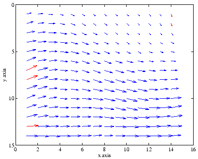
Figure 1 shows the calculated velocity vectors using the cross-correlation algorithm with a $64\times64$ pixel window size, one time recursive (reducing the window size by one half) and 50% overlap between adjacent windows. The blue arrows in the figure indicate the estimated velocity vectors while the red arrows indicate the interpolated velocity vectors that replace the eliminated spurious vectors by mpiv_filter.m.

If your MATLAB version is higher than 6.5 (R13) running on MS Windows system, GUI menu is available for demonstration.

>> mpiv_gui

GUI menu will be popped up. Please select adequate parameters for velocity estimation.

A typical flow chart for running mpiv can be summarized as follows.

1. read in sequential images (using, e.g., `imread').
2. Estimate velocity vectors using mpiv.m.
3. Remove error vectors and replace them by interpolation using mpiv_filter.m.

That is all (and hopefully simple)!

Figure 1: Result from mpiv_filter.m. Error vectors correction and interpolation: blue, original output; red, interpolated after removing error vectors.