The visualization method is developed to measure both bubble shape and its moving velocity in a gas phase simultaneously.
The method is basically based on the shadow graph method (SGM, hereafter for simplicity) and particle tracking method.
Therefore, we denotes this method as Bubble Tracking Velocimetry or BTV for simplicity here after,
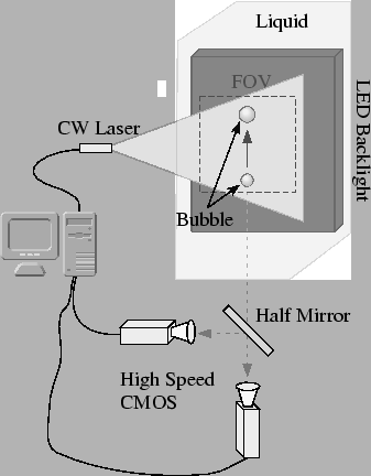
First, the bubble is projected into the vertical two dimensional domain by the shadow graph method using a flat back light.
The back light gives clear shadow image of the bubble or bulk of air, although it is a two dimensional projection from a three dimensional bubble shape.
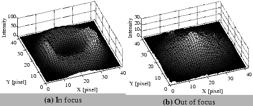
Fig.![[*]](crossref.png) shows examples of captured bubble image both in and out focus by SGM.
The in focus captured bubble image as shown in Fig. (a) shows clear edge of the bubble.
The projected bubble shape can be calculated by tracing the edge.
However, the out of focus bubble image as shown in Fig. (b) has no clear boarder on the edge and is hard to analyze.
Although the actual edge is slightly larger than observed edge owing to the refraction of the light, the refraction of the light through the bubble is neglected in here.
The captured bubble image has exact location within the thickness of focus range
that is 30cm approximately in this setup.
Secondary, the traced edge bubbles are approximated by elliptic curves.
The major and minor axes, and angles of the axis are estimated by the least-square method.
The estimated error depends on the number of pixels of bubble image and is 2% approximately confirmed by the numerical simulation.
Finally, the bubble moving velocity is estimated by the conventional three time particle tracking method.
This is an extension of the particle tracking velocimetry using the bubble as a tracer.
Thus, this method denotes bubble tracking velocimetry, BTV, hereafter for simplicity.
shows examples of captured bubble image both in and out focus by SGM.
The in focus captured bubble image as shown in Fig. (a) shows clear edge of the bubble.
The projected bubble shape can be calculated by tracing the edge.
However, the out of focus bubble image as shown in Fig. (b) has no clear boarder on the edge and is hard to analyze.
Although the actual edge is slightly larger than observed edge owing to the refraction of the light, the refraction of the light through the bubble is neglected in here.
The captured bubble image has exact location within the thickness of focus range
that is 30cm approximately in this setup.
Secondary, the traced edge bubbles are approximated by elliptic curves.
The major and minor axes, and angles of the axis are estimated by the least-square method.
The estimated error depends on the number of pixels of bubble image and is 2% approximately confirmed by the numerical simulation.
Finally, the bubble moving velocity is estimated by the conventional three time particle tracking method.
This is an extension of the particle tracking velocimetry using the bubble as a tracer.
Thus, this method denotes bubble tracking velocimetry, BTV, hereafter for simplicity.
The image processing procedure of BTV can be summarized as follows (see Fig.): The background of the images was removed, first.
Then original bubble shape is extracted by the edge detection.
After that, the elliptic approximation of bubble shape is calculated and the major, minor and angle of the elliptic shape bubble are estimated to avoid sub-pixel error.
Finally the bubble velocity is estimated by the particle tracking method (PTV).
Basically, the PTV is applied for the bubble velocity estimation but the particle image velocimetry (PIV) without bubble shape estimation is applied for the highly dense entrapped air area owing to the overlapped bubble image.
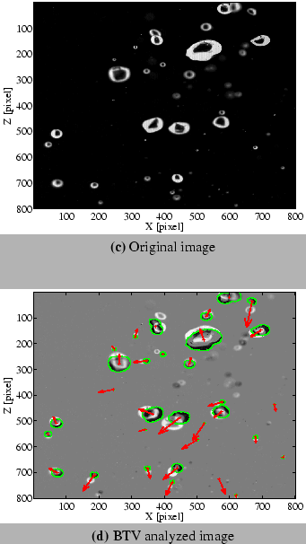
Fig. shows example of BTV method.
Fig. (a) is the original image and (b) is the BTV analyzed image.
The BTV analyzed image shows bubble shape of in focus bubble and velocity.
The BTV can be estimated 2D projected bubble shape and velocity within 10cm![]() 10cm area simultaneously.
This is impossible using a standard in-situ probe.
10cm area simultaneously.
This is impossible using a standard in-situ probe.