Experimental Setup

A flat LED light (10cm$\times$10cm) was used for the shadow graph to avoid flicker of the back light. A continuous diode laser operated at a power of 5W and a wavelength of 532 nm was used as the light source to adjust the exact location of bubble in transverse direction of bubble between the camera and the back light. A cylindrical lens mounted in front of the laser was used to create the light sheet. An 8-bit high speed CMOS camera with a resolution of 1280$\times$1024 pixels was used to capture the images. The images were captured at a framing rate of 125-250 frames per second. Each captured image was stored in a PC and later analyzed using the BTV image processing technique with results similar to those shown in Fig.. The uncertainty owing to image distortion was also checked using fixed markers in the tank and found that the maximum error was 1.5 mm (about 5 pixels). Fig. shows the sample of BTV experimental setup using two cameras. The half mirror was used to divide one image into two cameras. The two cameras can be installed different lens to enhance the resolution of field of view (FOV). However, only one camera was used in this study.

Figure: Illustration of experimental setup

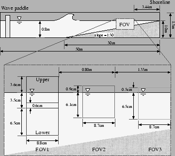
The breaking wave experiments were conducted in a wave tank that is 50.0 m long, 1.0 m wide, and 1.5 m deep located in Osaka City University. The one side wall of the tank was constructed using glass for optical access. The BTV imaging system shown in Fig. was set up in the middle of the tank. A fixed, impermeable 1/30 slope was installed with the toe 20 from the wavemaker. The water depth was 1.0 m, and regular wave trains were generated by a computer-controlled piston-type wavemaker with active absorber A detail of the experimental setup is shown in Fig.

Figure: Time history of void fraction (solid line: void fraction, dashed line: area of liquid in the image)

The three different locations were chosen as field of view (FOV) of the BTV measurements. The FOV 1-3 were located at $3h_b$, $7h_b$ and $15h_b$, respectively. Here $h_b$ denotes the water depth at the breaking point (B.P.). The void fraction in this study is defined by the spatial ratio to bulk of air and water below the free surface. Therefore, the location of the free surface becomes important to define the void fraction. The edge detection method as same as bubble shape detection was used to identify the free surface. The threshold value of edge detection for the free surface was selected through the trial and error through the checking process.

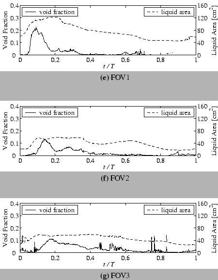
Fig. shows an example of the instantaneous time series of void fraction measured by the BTV. The solid and dashed line denote void fraction, and area of liquid in the image. The spatial-averaged void fractions do not decreased monotonically as () investigated. This is because the difference between the instantaneous (BTV measured) and phase-averaged void fraction (void fraction measured). The measured time series of void fraction have several interesting characteristics, although measurement locations were limited to discuss in detail. First, the maximum values of void fraction were decreased as breaking wave propagates to shoreline (FOV1 $\rightarrow$ FOV3). The void fraction at FOV1 ($x=3h_b$) exceeds 0.2 but is about 0.1 at FOV3 ($x=15h_b$). Second, the rising up of void fraction from 0 to the maximum at FOV1 is faster than the others and is decreased as FOV1 $\rightarrow$ FOV3. In addition, the decreasing rates of void fraction after reached maximum value show the similar tendency. Thus, the bulk of air was massively injected into the water near the B.P. and was diffused as wave propagated to shoreline. The BTV can be measured these characteristics from the spatial-averaged (depth-averaged) point of view.

Figure: Time series of bubble size distribution

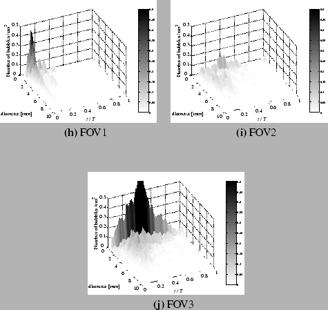
Fig. shows the time series of bubble diameter distribution. The bubble diameter denotes mean value of major and minor diameter of elliptic approximation of 2D projected plane. The horizontal axes are time normalized by the incident wave period and the characteristics diameter. The vertical axis is number of bubbles per unit area. The bubble number density usually has a dimension of [Number of bubbles/ m$^{-4}$] but the BTV is 2D measurement therefore the bubble number density is normalized by unit area. As already shown in Fig., the bulk of air injected into the free surface rapidly and decreased near the breaking point (FOV1) rather than far field (FOV3). The time series of the bubble number density distribution, Fig., shows similar tendency but the number of small scale bubble has different behavior. Generally, entrapped air by breaking waves is split into small bubbles owing to the shear and turbulence of surrounding flows. The early work of this problem for a general condition discussed by () and () in the middle of the last century and a large bibliography has been generated (i.e. , ). The bubble size spectra in FOV1 and 3 show two clear peaks, but the appeared time of peaks is different as shown in Fig. (a) and (c). The number of small size bubble smaller than 1mm increased significantly. The difference of the bubble size spectra between FOV1 and 3 can be explained by the bubble splitting owing to strong shear flow generated by the breaking waves. The detail of small scale bubble characteristics related with the power-law scaling of bubble size spectra is discussed next.

Figure: Power law of bubble size distribution

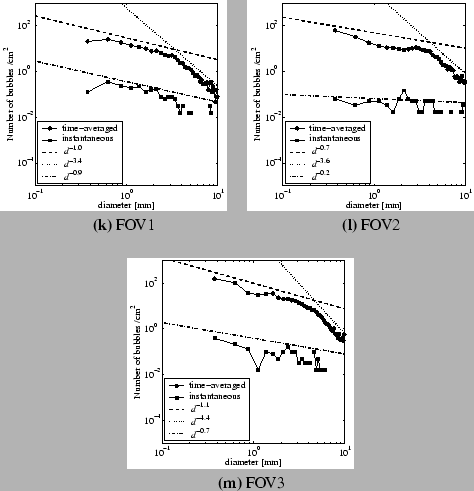
To check the power-law scaling of the bubble size spectra in the surf zone, Fig. shows the instantaneous and time-averaged bubble size spectra with the estimated power-law by the least-square method. The instantaneous bubble size spectra corresponds at the time of the maximum void fraction. There are two scaling laws can be seen at all FOVs. The small and large size bubble power scaling laws are $d^{-0.7\sim-1.1}$ and $d^{-3.4\sim-4.4}$, respectively. There is no significant difference between instantaneous and time-averaged spectra. The critical point in between two power scaling corresponds to the Hinze scale of bubble splitting theory (, ). () proposed semi-empirical $-10/3$ power-law scaling for the bubble which is larger than the Hinze scale based on the discussion of bubble fragmentation in the strong turbulence flow below the trough level. The measured power-law scaling of large size bubble size spectra is similar to (). On the other hand, () measured a $-3/2$ power-law scaling, smaller than the Hinze scale (1mm) of the acoustically active phase near the crest. The power-law scaling of small size bubble shown in Fig. is close to $-3/2$ power-law predicted by (). The Hinze scale of time-averaged spectra at FOV1 is smaller than FOV3. This is related with the turbulent intensity and energy dissipation induced by the breaking waves. The detail mechanisms and relationship between the Hinze scale and energy dissipation require liquid phase measurements and should keep for future study.