Surface wave profile and wave statistics

It is important for engineering practice to make clear the high-order nonlinear effects on water surface elevations and their statistics, because understanding of the wave characteristics/statistics is valuable for engineering. Figure 5 shows the spatial wave profiles of the high-order and 2nd order solutions at the evolution time of $t/T_p$=25 for $m$=10 and $k_ph$=$\infty$. The whole of the surface profiles of the high-order and second-order solution is quite similar, however, a giant and steep wave, a freak wave like, can be observed at $k_px$=140 of the high-order solution. It is found that the high-order nonlinear interactions is strongly related to the occurrence of a single extreme wave having the outstanding crest height, because such wave can never be observed in the second-order nonlinear solution. The occurrence of the steep wave is related to higher wavenumber components than 2$k/k_p$.

Figure 6: Temporal histories of $GF$ of simulated wave train both of high-order solution and second-order one(solid line: high-order solution, dashed line: second-order solution, filled circle:$m$=10, filled triangle:$m$=30, respectively).cont.

Figure 6: Temporal histories of $GF$ of simulated wave train both of high-order solution and second-order one(solid line: high-order solution, dashed line: second-order solution, filled circle:$m$=10, filled triangle:$m$=30, respectively).

The fact that the high-order nonlinear interactions generate the steep wave suggests that such high-order nonlinearities also affect on wave statistics. Thus $GF$ (Groupiness Factor) is picked up to describe the characteristics of wave train. The time histories of $GF$ during the propagating process are shown in Figure 6 for $m$=10, 30 and 100. $GF$ of the non-linear solution are always larger than the second non-linear solution, and the high-order effects is strong for initially narrow banded spectrum wave in deep-water condition. Moreover, if the water depth becomes shallower, differences between the high-order and the second-order solution become small. And finally they are almost the same in the case of $k_ph$=1.36 that is equal to a saddle node point of the stability of the nonlinear schrödinger equation.

Figure 7: Time averaged wave statistics as a function of spectrum bandwidth $m$ in deep-water condition(solid line:high-order solution, dashed line:second-order solution).

Figure 8: Time averaged wave statistics as a function of relative water depth $k_ph$ for $m$=4, 10, 30(solid line:high-order solution, dashed line:second-order solution, filled circle:$m$=4, filled triangle:$m$=10, filled square:$m$=30, respectively).

Figure 9: Comparison of exceedance probabilities of wave heights among high-order solution, second-order one and the Rayleigh distribution.

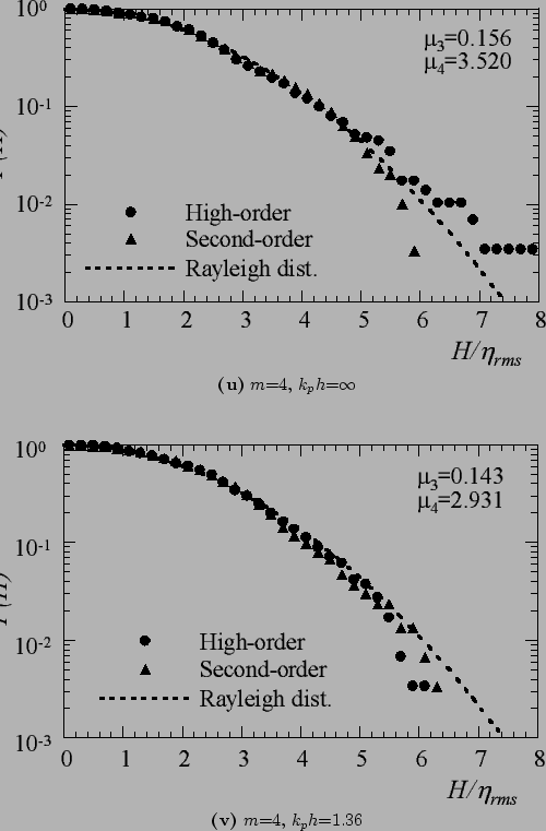To verify the effects of the high-order nonlinearities on wave statistics quantitatively, time averaged $GF$, $H_{max}/H_{1/3}$, kurtosis:$\mu_4$ and skewness:$\mu_3$ are plotted in Figure 7 and Figure 8 as a function of initial spectrum band width $m$ and water-depth $k_ph$, respectively. The vertical bars in the figures indicate variance of the statistics and bracket$<>$ indicates time averaged value. The difference of between the high-order and the second-order solution is small. However, , and of the high-order solutions are larger than the second-order solution, and the differences between the high-order solution and the second-order one are decreased if the spectrum band width becomes broader in deep-water. These differences are decreased in $k_ph$=2.0 and vanished in $k_ph$=1.36. Moreover, they have opposite relationship in $k_ph$=1.0. This imply that the high-order nonlinear effects play an important role to stabilize the waves in shallow-water. The effects of the high-order nonlinearities are the most remarkable in $\mu_4$. The reason why $\mu_4$ stands out is that $\mu_4$ depends on the third-order nonlinearities in statistically (Longuet-Higgins, 1963). Therefore, the value of $\mu_4$ is one of the milestones to check the influence of the high-order nonlinearities of the observed wave train.