Next: Wave Height Distributions
Up: Mathematical formulations
Previous: Mathematical formulations
We assume that waves to be analyzed here are unidirectional with narrow banded spectra and satisfy the stationary and ergodic hypothesis.
Let  be the sea surface elevation as a function of
  and
and  be its Hilbert transform.
Assuming both
be its Hilbert transform.
Assuming both  and
and  are real zero-mean function with variance
  , we have
The characteristic function  can be described as
![\begin{displaymath}
\psi_z(u,v) = E\left[e^{i(u\eta+v\zeta)}\right],
\end{displaymath}](img17.png) |
(4) |
where ![$E[\cdot]$](img18.png) means the expected value operator, and
means the expected value operator, and  and
and  are dummy variables in
 .
.
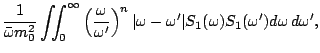
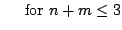
The cumulants  is formulated by Eq.(4) as
 |
(5) |
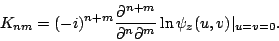
The following relationship is established between the characteristic function  and cumulant .
between them, so we have
and cumulant .
between them, so we have
![\begin{displaymath}
\psi_z(u,v) = \exp\left[
\sum_{n}\sum_{m} \frac{K_{nm}}{n!m!}
(iu)^n(iv)^m
\right].
\end{displaymath}](img25.png) |
(6) |
Longuet-Higgins (1963) formulated the detailed relationship between Eq.(5) and Eq.(6).
Several values of cumulants are derived from Eq.(5) on the basic assumptions, stationariness and orthogonal property of and .
 |
 |
![$\displaystyle E[\eta ] = \bar{\eta } = 0$](img27.png) |
(7) |
 |
|
![$\displaystyle E[\zeta] = \bar{\zeta} = 0$](img29.png) |
(8) |
 |
|
![$\displaystyle E[\eta^2] = \eta_{rms}^2$](img31.png) |
(9) |
 |
|
![$\displaystyle E[\eta\zeta] = 0$](img33.png) |
(10) |
 |
|
![$\displaystyle E[\eta^n\zeta^m]$](img35.png) |
|
| |
|
 |
(11) |
|
|
![$\displaystyle E[\eta^n\zeta^m] + (n-1)(m-1)(-1)^{n/2}\sigma^{n+m}$](img37.png) |
|
| |
|
 |
(12) |
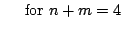
Similar results can be extended for the higher order cumulants, but the analysis is not carried out here beyond the fourth order.
Mori and Yasuda (1994) pointed out that the fourth order moment of water surface elevation is a dominative parameter for wave height statistics.
In present case, therefore, we should take into consideration up to the fourth order cumulants.
The joint probability density function of and is formulated as
where
and  is the
  th order Hermite polynomial expressed as
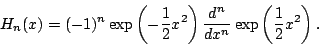 |
(17) |
It is noticed here that  =
= =
= =
= =0,
=0,  =
=  =1 and
  =
= =
= =
= =0, which have already been used in Eq.(7).
 is equal to the skewness
  of and
  is equal to kurtosis
  .
There is still unknown cumulants such as
.
There is still unknown cumulants such as  ,
,  ,
,  .
.
Tayfun (1993) formulated for weakly nonlinear waves wtih narrow banded spectra using the second order kernel function in deep water as,
where  is the mean angular frequency of spectrum and
  is sum of spectrum of the first order component.
By way of Schwarz's inequality an equality,
 is derived.
This gives
is derived.
This gives
 |
(20) |
and
 |
(21) |
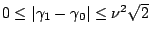
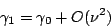
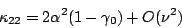
Since, the maximum value of is  , it is assumed there that =0 and also = and = under the condition of weak nonlinearlity.
Next: Wave Height Distributions
Up: Mathematical formulations
Previous: Mathematical formulations
2005-11-21
![$\displaystyle p(\eta',\zeta') =
\frac{1}{2\pi}\exp\left[-\frac{1}{2}(\eta'^{2}+\zeta'^{2})\right]$](img39.png)
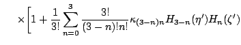
![$\displaystyle \hspace{0.75cm}
+ \frac{1}{4!}\sum_{n=0}^{4}
\frac{4!}{(4-n)!n!}\kappa_{(4-n)n}
H_{4-n}(\eta')H_{n}(\zeta')
\biggr]$](img41.png)