Let ![]() =
= ![]() and transform of variables from
and transform of variables from ![]() to
to
![]() express the joint probability density of the envelope
express the joint probability density of the envelope ![]() and
and ![]() in the form.
in the form.
Transformation of Eq.(22) by Eq.(23) and its integration with regard to ![]() over [
over [![]() ] yield the local wave amplitude distribution.
] yield the local wave amplitude distribution.
Eq.(24) is the distribution with the parameters of ![]() and
and ![]() and agrees to the Rayleigh distribution.
This states that Eq.(24) could be treated as an extended distribution of the Rayleigh distribution.
Therefore, we should call Eq.(24) as the Edgeworth-Rayleigh distribution(or ER distribution).
and agrees to the Rayleigh distribution.
This states that Eq.(24) could be treated as an extended distribution of the Rayleigh distribution.
Therefore, we should call Eq.(24) as the Edgeworth-Rayleigh distribution(or ER distribution).
Assuming a weakly nonlinearity and narrow banded spectrum enables us to treat wave height ![]() as two times of wave amplitude
as two times of wave amplitude ![]() , that is,
, that is, ![]() = 2
= 2![]() .
Then the wave height distribution is calculated by Eq.(24).
.
Then the wave height distribution is calculated by Eq.(24).
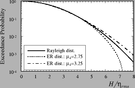
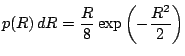
The exceedance probability of wave heights is given by integrating Eq.(26) over the range of ![]() :
:
2 shows the exceedance probability of the wave heights for the case of
![]() =2.75 and 3.25 with
=2.75 and 3.25 with
![]() =0.
The occurrence probability of the larger wave heights exceeds that of the Rayleigh distribution is increased when the value of
=0.
The occurrence probability of the larger wave heights exceeds that of the Rayleigh distribution is increased when the value of
![]() is larger than 3.
The value of kurtosis is dominated parameter for the PDF of wave heights.
is larger than 3.
The value of kurtosis is dominated parameter for the PDF of wave heights.
![$\displaystyle p(\eta,\zeta) =
\frac{1}{2\pi}\exp\left[-\frac{1}{2}(\eta^{2}+\zeta^{2})\right]$](img78.png)
![$\displaystyle \hspace{0.5cm}
\times
\biggl[
1 + \frac{\kappa_{30}}{6}H_3(\eta)
+ \frac{\kappa_{40}}{24}H_4(\eta)
+ \frac{\kappa_{30}^2}{24}H_6(\eta)
\biggr]$](img79.png)
![$\displaystyle \hspace{0.5cm}
\times
\biggl[
1 + \frac{\kappa_{03}}{6}H_3(\zeta)
+ \frac{\kappa_{04}}{24}H_4(\zeta)
+ \frac{\kappa_{03}^2}{24}H_6(\zeta)
\biggr]$](img80.png)
![$\displaystyle \hspace{0.5cm}
\times
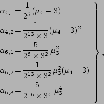
\left[ 1+\sum_{i=1}^{2}\alpha_{4,i}A_{4,i}(R)
+\sum_{i=1}^{3}\alpha_{6,i}A_{6,i}(R)
\right]
dR,$](img90.png)
![\begin{displaymath}
p(H') dH' = \frac{H'}{4}
\exp\left(-\frac{H'^2}{8}\righ...
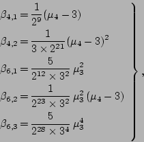
...eft[ 1 + \sum_{i,j}\beta_{i,j}B_{i,j}(H')
\right] dH',
\end{displaymath}](img97.png)
![\begin{displaymath}
P(H)=\exp\left(-\frac{H^2}{8}\right)
\!\left[ 1 + \sum_{i,j}\beta_{i,j}E_{i,j}(H)\right]\!,
\end{displaymath}](img104.png)