First, it is assumed unidirectional, stationarity and ergodicity for
wave field.
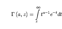
The most widely used statistical distribution describing wave height and
crest/trough amplitude is the Weibull distribution.
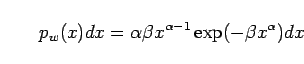
As a starting point of this study, it is assumed that the PDF of
wave/crest height can be described by the Weibull distribution
(Kendall and Stuart, 1963) given by
For the deck overtopping problem, the wave crest amplitude is the
dominant variable compared with either the wave trough amplitude
or wave height, although wave period is also important for overtopping.
Moreover, the wave nonlinearities enhance vertical asymmetry of waves,
and, as a result, the wave crest amplitude is
generally larger than its trough amplitude.
Therefore, only Eq.(1) for the PDF of wave crest
amplitude is used hereafter. This implies that for fixed ![]() =1/2,
=1/2,
![]() is the only empirical parameter
controlling profile of the distribution.
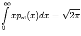
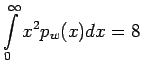
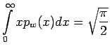
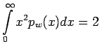
The mean and rms value of Eq.(1) with
is the only empirical parameter
controlling profile of the distribution.
The mean and rms value of Eq.(1) with ![]() are given by
are given by
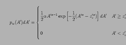
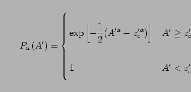
If the deck is thin compared to the incident wave amplitude, then
the influence of the
deck on the incident wave profile is negligible.
In this case, the PDF of the wave amplitude distribution on the deck can
be described by a truncated form of Eq.(1):
The same number of waves in Eq.(9) and
Eq.(10) is used in Eq.(1).
Therefore, the small amplitude wave which is smaller than ![]() is also
taken into consideration in in Eq.(9) and Eq.(10).
Obviously, the equivalence assumption of
is also
taken into consideration in in Eq.(9) and Eq.(10).
Obviously, the equivalence assumption of ![]() between
Eq.(1) and Eq.(9) depends on the thickness of
the deck in comparison with the incident wave height and wave nonlinearity.
The effect of the structure on the total wave height is minimal,
if the deck is thin and has little influence on the incident wave.
On the other hand,
between
Eq.(1) and Eq.(9) depends on the thickness of
the deck in comparison with the incident wave height and wave nonlinearity.
The effect of the structure on the total wave height is minimal,
if the deck is thin and has little influence on the incident wave.
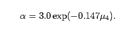
On the other hand, ![]() , is to be determined empirically.
Mori (2003) used experimental data to
investigate the relationship between
, is to be determined empirically.
Mori (2003) used experimental data to
investigate the relationship between ![]() and the kurtosis,
and the kurtosis,
![]() , of the surface elevation for deep-water random waves.
The regression curve given by Mori (2003) is
, of the surface elevation for deep-water random waves.
The regression curve given by Mori (2003) is
|
=11cm
![\includegraphics[width=11cm]{figures/exp_amp_offdeck_pdf_case1.eps}](img74.png)
(a) Case 1.
=11cm ![\includegraphics[width=11cm]{figures/exp_amp_offdeck_pdf_case2.eps}](img75.png)
(b) Case 2. |
Fig.4 compares the measured PDF of normalized wave crest
amplitudes with the computed PDFs for the Rayleigh amplitude
distribution and the Weibull amplitude distribution, Eq.(1).
The kurtosis values of the incident waves were about 3.4 and 3.3,
respectively (Table 1).
Therefore, the incident wave field was highly nonlinear compared
to observations of real ocean waves.
This difference may be to due to three dimensional or wind effects
not present in the hydraulic model study.
Since the values of ![]() were smaller than 2.0,
the peak of the Weibull distribution is lower than that of the Rayleigh
distribution, and the tail of the Weibull distribution is higher.
The Weibull distribution gives an overall better fit to the
experimental data compared to the Rayleigh distribution.
were smaller than 2.0,
the peak of the Weibull distribution is lower than that of the Rayleigh
distribution, and the tail of the Weibull distribution is higher.
The Weibull distribution gives an overall better fit to the
experimental data compared to the Rayleigh distribution.
|
=11cm
![\includegraphics[width=11cm]{figures/exp_amp_exc_case1.eps}](img78.png)
(a) Case 1.
=11cm ![\includegraphics[width=11cm]{figures/exp_amp_exc_case2.eps}](img79.png)
(b) Case 2. |
Fig.5 compares the exceedance probability of the
normalized wave crest amplitude for the experimental results at Gage 1 and 2
with the Rayleigh and Weibull distributions for Case 1 and 2.
The exceedance probability of the Weibull distribution is calculated by
Eq.(10) and the Rayleigh distribution is calculated by
Eq.(10) with ![]() .
The Weibull distribution gives better agreement to the
experimental data for the seaward location (Gage 1) for both cases
and for the waves on the deck (Gage 2) for the lower deck case (Case 1).
For the higher deck case (Case 2), the experimental data is located in
between that of the Weibull and Rayleigh distributions on the deck.
.
The Weibull distribution gives better agreement to the
experimental data for the seaward location (Gage 1) for both cases
and for the waves on the deck (Gage 2) for the lower deck case (Case 1).
For the higher deck case (Case 2), the experimental data is located in
between that of the Weibull and Rayleigh distributions on the deck.
![\includegraphics[width=10.0cm]{figures/overtopping_illustration2.eps}](img69.png)